Using Radio Buttons to Change Displayed Data

The vast majority of the workbooks that I do for customers are not printed but are used to interactively display data.  A good example of this would be a workbook that displays Sales data by Branch.  Select a Branch and Period and the workbook displays the data change the Branch and data for the new Branch is displayed.  There are occasions where the user wants to be able to easily change the data that's being displayed from one type to another.  An example would be providing the ability to switch between Gross Margin based on Replacement Cost and Gross Margin based on Weighted Average Cost.  One way to accomplish this is by using Radio Buttons.  Excel has two different types of Radio Buttons, Active-X and Forms; we'll be looking at the Forms type in this post.


We'll use the table below as the data source for our workbook

Select another worksheet and for Excel 2007 click the Developer tab and then from the Controls section click Insert and then click the Radio Button (Option Button) under Forms Control.

Click on the active worksheet in the general area where you want the Radio Button and Excel will create the Button as below.  For our purposes we'll not use the Caption so right click on the Button and select Edit Text and delete the text.

Right click and Copy the Button then right click and Past to create a second Button.

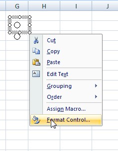
Right click on one of the Buttons and click Format Control.

Click in the Cell link box and then click in cell L2 and then click OK.  This links the buttons to cell L2.

Now, click one of the buttons and a number will appear in cell L2.  Click the other button and the number will change.  Since we have two buttons the numbers will be 1 and 2 and will change depending on the button that is active.  We can now reference cell L2 in a formula in order to display different results for our worksheet.


In cell B2 enter "Sales".  In cell B3 enter =Sheet1!A2 and then copy to cells B4 and B5.  In cell C3 enter =IF($L$2=1,Sheet1!D2,Sheet1!E2) and then copy to cells C4 and C5.  In cell D3 enter =IF($L$2=1,Sheet1!F2,Sheet1!G2) and copy to cells D4 and D5.  Format the data as desired and you should have something like this:

Since the data can change then we need to change the headings to match.  In cell C2 enter ="GM$ at "&IF($L$2=1,"RC","WAC") and in cell D2 enter 
="GM% at "&IF($L$2=1,"RC","WAC").  In cells H2 enter "Replacement Cost" and in cell H3 enter "W.A.C."


Format the headers as desired and you should have something similar to this:

As always, if you have any questions or comments leave them here or email me at the office.