This workbook displays a Moving Average Sales Forecast by Branch for either Sales or Gross Margin. The data displayed changes when the Branch Number is changed
Thursday, April 28, 2011
Wednesday, April 27, 2011
Workbooks Being Used by Our Customers
SALES WITH METHOD OF PAYMENT
This workbook was designed to show key information regarding Cash Sales. Included are the following:
Cash Sales as % of Total Sales
Method of Payment for Cash Sales
Method of Payment for DepositsCREDIT MEMO'S BY REASON CODE
This workbook displays Amount and % of Total by Reason Code for Selected Period or Range of Periods.
When the Code Descriptions button is clicked a list of valid Codes with Descriptions is displayed. When the button is clicked again the Descriptions are hidden.
Selection by Branch, Region or ALL
Here's a way to use a Combo Box to select a Branch or range of Branches the result of which can be passed to an MS Parameter Query.
To begin enter data as below in a worksheet.
Select the cells from A2 to A18 and in click in the Name Box (immediately above column A) and type BranchList (no space between Branch and List) and press enter.
Now Select cells B2 to C18 and type BranchData in the name box.
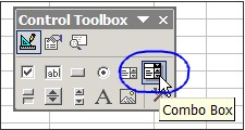 A Combo Box will allow us to return a numeric value to a specified cell based the selection made int the Box and also allows us to specify the range of cells to be used for the input. For Excel 2003 click View > Toolbars > Forms to display the Forms Tool Bar. In Excel 2007 click the Developer tab on the Ribbon and then Insert Forms. Click the Combo Box icon and then on your worksheet click in the area where you want to place the Combo Box. Adjust the size of the by dragging the corners or edges.
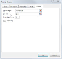 Right click on the Combo Box and select Format control. Click the Control tab and type BranchList in the Input range box. Type $E$1 in the Cell link box. Check the 3-D shading. Click OK
In cell F5 type From Branch. In cell G5 type To Branch. In cell F6 enter =INDEX(BranchData,$E$1,1) and in cell G6 enter =INDEX(BranchData, $E$1,2).
Now when a selection is made in Combo Box the values under From Branch and To Branch should change to match the values in Columns B and C that correspond to the value in Column A
To begin enter data as below in a worksheet.
Select the cells from A2 to A18 and in click in the Name Box (immediately above column A) and type BranchList (no space between Branch and List) and press enter.
Now Select cells B2 to C18 and type BranchData in the name box.
This creates two named ranges that will be used to create the From and To Branch numbers that can be passed as parameters to MS Query. All that we're doing with this table is creating a beginning and ending Branch Number.
To extract the beginning and ending numbers for a specific value in column A we'll use the INDEX function. The arguments for the INDEX function are array (range of cells), row number and column number. Our array is the range B2:C18 (which we've named BranchData), the beginning branch is in column 1 of this array and the ending branch is in column 2. The row number is equal to the location of the entry in column A. The formula to return the beginning branch for ALL would be =INDEX(BranchData,1,1) and the formula for the ending branch would be =INDEX(BranchData,1,2). Since the beginning branch is always in column one and the ending branch is always in column 2 then all we need is a way to change the row value based on the selection from Column A (BranchList). To accomplish this we'll use a Combo Box.
 A Combo Box will allow us to return a numeric value to a specified cell based the selection made int the Box and also allows us to specify the range of cells to be used for the input. For Excel 2003 click View > Toolbars > Forms to display the Forms Tool Bar. In Excel 2007 click the Developer tab on the Ribbon and then Insert Forms. Click the Combo Box icon and then on your worksheet click in the area where you want to place the Combo Box. Adjust the size of the by dragging the corners or edges.
  Right click on the Combo Box and select Format control. Click the Control tab and type BranchList in the Input range box. Type $E$1 in the Cell link box. Check the 3-D shading. Click OK
In cell F5 type From Branch. In cell G5 type To Branch. In cell F6 enter =INDEX(BranchData,$E$1,1) and in cell G6 enter =INDEX(BranchData, $E$1,2).
Now when a selection is made in Combo Box the values under From Branch and To Branch should change to match the values in Columns B and C that correspond to the value in Column A
Sunday, April 24, 2011
Joining Two HD Files in MS Query
Open a new workbook and open MS Query. Select the Customer Balance file (ARPMBAL) and click add (or just double click ARPMBAL in the "Add Tables" dialog box). Add the Customer Master file (ARPMCUS) as above and click "Close".
In this case the two file are automatically joined using the Customer Number (ARNO01). In some cases the files will not auto-join and it is necessary to make the join manually. This can be done by clicking the field to be used for the join in one file and dragging it to the same field in the second file. Files can also be joined by clicking Table > Joins. MS Query uses INNER joins by default. An INNER join will return only records that are found in both files.
Select Branch Number (ARNO16), Salesman ID (ARID01), Customer Number (ARNO01) and Customer Name (ARNM01) by double clicking the field in the File.
Click Criteria > Add Criteria, click the dropdown and select ARPMCUS.ARFL10 or simply type ARFL10 in the Field box. Select "does not equal" in the Operator box and type a capital C in the Value box. Click Add and then Close
Click Records > Sort and select fields by which you want to sort the data. The order in which the records will be sorted can also be chosen. Click Add as each field is selected and when complete click Close.
Run the query to display the data that will be returned to the workbook.
Return the data to Excel and format as desired.
Friday, April 22, 2011
Working with HD Date Fields
If you've worked with the date fields in HD previously you're aware that HD does not use actual date fields but uses numeric fields for century, year, month and day. For accounting periods the day field is excluded.
In this example we'll use the Invoice and Sales Period date fields from the Invoice Header file (OEPTOHY). The Invoice fields are OECC01 (century), OEYR01 (year), OEMO01 (month) and OEDY01 (day). The Sales Period fields are OECC08 (century), OEYR08 (year) and OEMO08 (month)
Below data is being pulled from the Invoice Header file in HD. The Order Number, Invoice date fields and the Sales Period date fields have been selected. The century and year fields for both Invoice date and Sales Period have been combined to create create a "standard" year field. This could also be done after the data is returned to Excel. The formula is century times 100 plus the year (OECC01*100+OEYR01).
Here the data has been returned and the DATE function used to create a date from the HD fields. For the Inv Date the formula is =DATE(B2,C2,D2). Default formatting was used for Inv Date. For the Sales Period the formula is =DATE(E2,F2,1). The 1 is used for the day argument because Accounting Periods in HD have no Day field. Formatting for Sales Prd was changed to display only month and year.
Tuesday, April 19, 2011
Extracting Data from the Production Database
The following will allow you to extract data from a single file in HD. The following requires that an ODBC connection is already available on your PC.
For Excel 2003 click Data > Get External Data > New Database Query
For Excel 2007 click the Data Tab > From Other Sources > From Microsoft Query
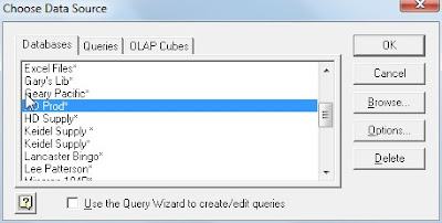
The Choose Date Source dialog box will display. Select the data source and click OK.
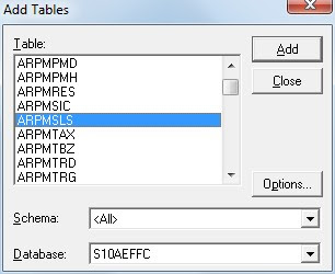
The Add Tables dialog box will display. Select ARPMSLS and click Add
The Salesman Master file (ARPMSLS) will be added. Select ARID01 (Salesman ID) and ARNM06 (Salesman Name) by double clicking in the ARPMSLS box.
Note: If the query runs when each field is clicked then Automatic Query is enabled. To disable click Records and uncheck Automatic Query. You can also enter the field name directly into the boxes where ARID01 and ARNM06 are displayed below. When you click in one of these boxes a drop down arrow displays; the fields can also be selected from the drop down.
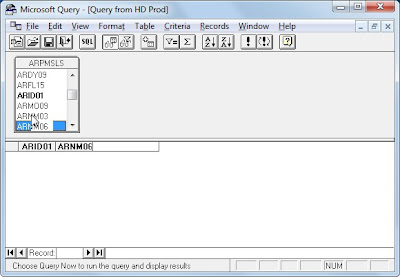
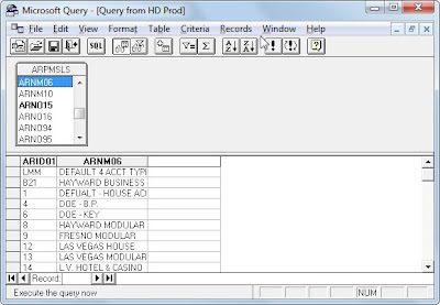
To display data from the file click Records > Query Now or click the "!" button. The records can be sorted by clicking Records > Sort. To add move the records to your workbook click File > Return Data to Microsoft Excel or click the fourth button from the left.
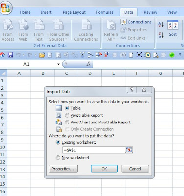
The Import Data dialog will display. Enter the location where you wish the data to begin on the worksheet or accept the default and click OK.
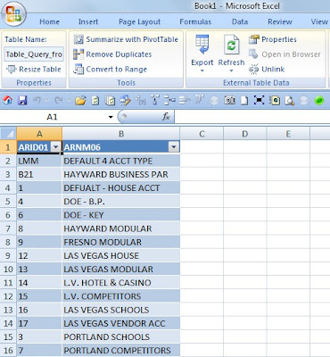
The data will now be loaded to your worksheet. The screen shot below is from Excel 2007 and will be different in Excel 2003.
For Excel 2003 click Data > Get External Data > New Database Query
For Excel 2007 click the Data Tab > From Other Sources > From Microsoft Query
The Choose Date Source dialog box will display. Select the data source and click OK.

The Add Tables dialog box will display. Select ARPMSLS and click Add

The Salesman Master file (ARPMSLS) will be added. Select ARID01 (Salesman ID) and ARNM06 (Salesman Name) by double clicking in the ARPMSLS box.
Note: If the query runs when each field is clicked then Automatic Query is enabled. To disable click Records and uncheck Automatic Query. You can also enter the field name directly into the boxes where ARID01 and ARNM06 are displayed below. When you click in one of these boxes a drop down arrow displays; the fields can also be selected from the drop down.

To display data from the file click Records > Query Now or click the "!" button. The records can be sorted by clicking Records > Sort. To add move the records to your workbook click File > Return Data to Microsoft Excel or click the fourth button from the left.

The Import Data dialog will display. Enter the location where you wish the data to begin on the worksheet or accept the default and click OK.

The data will now be loaded to your worksheet. The screen shot below is from Excel 2007 and will be different in Excel 2003.

ODBC Setup for HD Files
Click on Start > Control Panel > Administrative Tools > Data Sources (ODBC) to display the ODBC Data Source Administrator dialog box below
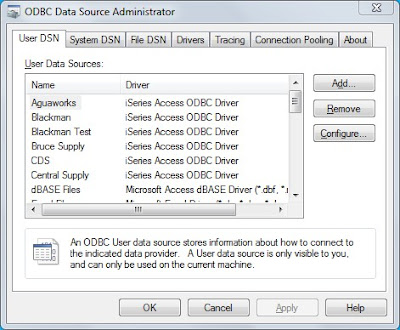
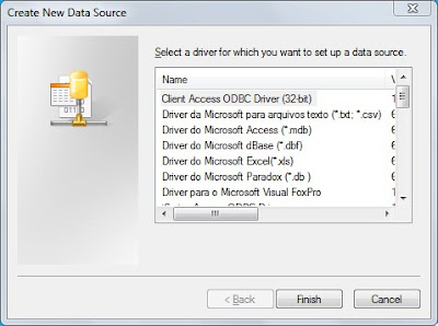

Click the “Add…” button to display the Create New Data Source dialog box below

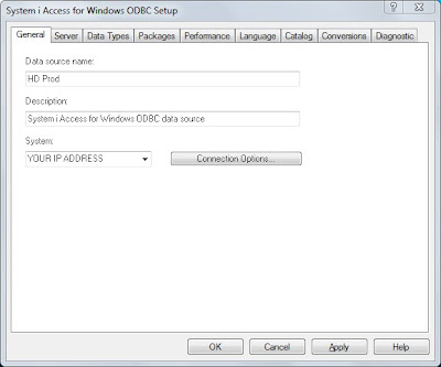
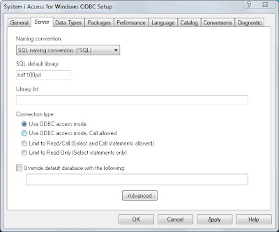
Select the either the “Client Access ODBC Driver” or the “iSeries Access ODBC Driver” and click “Finish” to display the System I Access for Windows ODBC Setup dialog box below. Type “HD Prod” in the” Data source name” box then click the Server tab

Type “HD1100PD” in the “SQL default library” box. Click “Apply” and then “OK” to complete the ODBC setup.

Sunday, April 17, 2011
Perpetual Date List for Data Validation
To create a list of twelve dates that do not have to be updated manually begin by entering the name of the list in Cell A1. For this example "validDates" has been used but any unique name will work. In cell A13 enter this formula - =TODAY(). In Cell A12 enter this formula = EDATE(A13,-1). Copy Cell A12 and Paste in Cells A2 thru A11.
Typically these dates will be used for as Month/Year (Billing Period, etc) so the day is not important. The cells containing the dates can now be formatted as desired (i.e. Apr-2011, April, 2011).
Now assign the list a name and it's ready to use for Validation. The quickest way to give the range a name is to select cells A2 thru A13 and then click in the "Name Box" (the box to the left of the Formula Bar that normally displays the address of the active cell) and type validDates or whatever name you prefer. Press enter and the entry is assigned to the range of cells.
The list of dates can now be used in for Data Validation by the assigned name.
Friday, April 15, 2011
Adding code to Personal Workbook
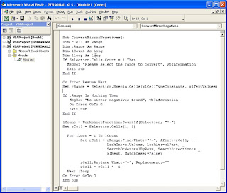 To add code to the Personal Workbook in Excel right click on any worksheet tab and click View Code to open the Visual Basic Editor.
If a Module already exists then copy and paste your code in to the Module. If no Module exists in the Personal Workbook then right click on the workbook in the Project explorer (Ctl +R to display explorer) > Insert > Module.
The code will now be available whenever Excel is open.
Thursday, April 14, 2011
Move Negative Sign
When importing data into Excel negative numbers may have the negative sign on the right side which will be viewed by Excel as text. The code below will move the sign to the left side.
Sub ConvertMirrorNegatives()
Dim rCell As Range
Dim rRange As Range
Dim lCount As Long
Dim lLoop As Long
If Selection.Cells.Count = 1 Then
MsgBox "Please select the range to convert", vbInformation
Exit Sub
End If
On Error Resume Next
Set rRange = Selection.SpecialCells(xlCellTypeConstants, xlTextValues)
If rRange Is Nothing Then
MsgBox "No mirror negatives found", vbInformation
On Error GoTo 0
Exit Sub
End If
lCount = WorksheetFunction.CountIf(Selection, "*-")
Set rCell = Selection.Cells(1, 1)
For lLoop = 1 To lCount
Set rCell = rRange.Find(What:="*-", After:=rCell, _
LookIn:=xlValues, LookAt:=xlPart, _
SearchOrder:=xlByRows, SearchDirection:= _
xlNext, MatchCase:=False)
rCell.Replace What:="-", Replacement:=""
rCell = rCell * -1
Next lLoop
On Error GoTo 0
End Sub
Subscribe to:
Comments (Atom)


