More On Using Radio Buttons

In the last post I failed to include how to add Radio Buttons in Excel 2003.  Select the worksheet where the buttons will be used and click View > Toolbars > Forms.  The toolbox below appears as a floating toolbar.

Then proceed as with Excel 2007.


Another thing that will come up when you begin using control buttons will be the need to use more than one set of buttons.  As we've seen multiple buttons use the same Cell Link and the number in the cell corresponds to the button that is active.  So whether you have two or twenty buttons they will all use the same cell and will increment based on the total number of buttons.


In order to have multiple sets of buttons it's necessary to use the Group Box from the Forms toolbar (below).

Click on the Group Box and then click on the worksheet and adjust the size of the box to include the buttons that are to be grouped together as below where buttons 1 & 2 are inside Group Box 6.

Buttons 1 and 2 can now be assigned to a different Cell Link.  Any buttons outside the Group Box can now be assigned to a different cell and will work independently of the buttons inside the box.

As always if you have any comments or question you can leave them here or email me at the office.

Using Radio Buttons to Change Displayed Data

The vast majority of the workbooks that I do for customers are not printed but are used to interactively display data.  A good example of this would be a workbook that displays Sales data by Branch.  Select a Branch and Period and the workbook displays the data change the Branch and data for the new Branch is displayed.  There are occasions where the user wants to be able to easily change the data that's being displayed from one type to another.  An example would be providing the ability to switch between Gross Margin based on Replacement Cost and Gross Margin based on Weighted Average Cost.  One way to accomplish this is by using Radio Buttons.  Excel has two different types of Radio Buttons, Active-X and Forms; we'll be looking at the Forms type in this post.


We'll use the table below as the data source for our workbook

Select another worksheet and for Excel 2007 click the Developer tab and then from the Controls section click Insert and then click the Radio Button (Option Button) under Forms Control.

Click on the active worksheet in the general area where you want the Radio Button and Excel will create the Button as below.  For our purposes we'll not use the Caption so right click on the Button and select Edit Text and delete the text.

Right click and Copy the Button then right click and Past to create a second Button.

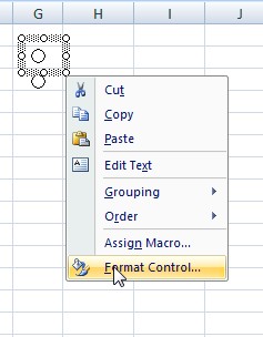
Right click on one of the Buttons and click Format Control.

Click in the Cell link box and then click in cell L2 and then click OK.  This links the buttons to cell L2.

Now, click one of the buttons and a number will appear in cell L2.  Click the other button and the number will change.  Since we have two buttons the numbers will be 1 and 2 and will change depending on the button that is active.  We can now reference cell L2 in a formula in order to display different results for our worksheet.


In cell B2 enter "Sales".  In cell B3 enter =Sheet1!A2 and then copy to cells B4 and B5.  In cell C3 enter =IF($L$2=1,Sheet1!D2,Sheet1!E2) and then copy to cells C4 and C5.  In cell D3 enter =IF($L$2=1,Sheet1!F2,Sheet1!G2) and copy to cells D4 and D5.  Format the data as desired and you should have something like this:

Since the data can change then we need to change the headings to match.  In cell C2 enter ="GM$ at "&IF($L$2=1,"RC","WAC") and in cell D2 enter 
="GM% at "&IF($L$2=1,"RC","WAC").  In cells H2 enter "Replacement Cost" and in cell H3 enter "W.A.C."


Format the headers as desired and you should have something similar to this:

As always, if you have any questions or comments leave them here or email me at the office.

Import JE Data into MyHD

One of the great new features in MyHD is the ability to easily import Journal Entry Data.  The user enters the G/L Account Number, Amount and Description in Excel and then saves as a .CSV file.  


The user simply navigates to the Journal Entry screen and enters the Journal Reference code and Reference Number then clicks OK.

The user now clicks the Import button

Selects the file to be imported

Click Open and the data is loaded to the JE

To make this process even simpler we've created an Excel workbook specifically for the data entry

This workbook has MS query that runs against the customers database and validates the G/L Accounts plus a formula to indicate that the data is in balance.  When the data entry is completed the user clicks the "Crt CSV" button and the data is copied to a new workbook which is then saved on the users C drive.

We also have a workbook for loading JE Data to the database for customers that are still using HD.  Since there is no Import feature in HD the data from the workbook is loaded to the database via Client Access.

If you would like a copy of either of these workbook send me an email and I'll forward it to you.

As always if you have any questions or comments you may post them here or email me directly.

Date Selections for HD Parameter Queries

I receive frequent requests for reports that require the user to provide a from and to date to the MS Query.  Ideally you would like to prevent the user from receiving an error message because a to date that is less than the from date is entered.  There are several way of accomplishing this and here is the one that I prefer.


Here's the layout of our sample workbook.

The todate list (column B) is built by entering =TODAY() in cell B13 and then entering =EOMONTH(B13,-1) in cell B12.  The formula in B12 is then copied and pasted in range B2:B11.  This populates the range B2:B12 with the last day of each month for the  previous 11 months.

The fromdate list (column A) is built by entering =DATE(YEAR(B2),MONTH(B2),1) in cell A2.  The formula is then copied  and pasted in the range B3:B13.  This populates the range A2:A13 with the first day of each month corresponding to the date in column B.

The Named Range "fromdate" is created by selecting the range A1:A13 and selecting  Formulas >  Create from Selection and clicking OK.

Select cell I2 and then Data > Data Validation and from the dropdown select List.  In the Source box enter =fromdate and click OK.  Cell I2 now has a drop down from which the user can select a date.  Format the cell with a date format.

Since the user should not be able to select a todate that is less than the fromdate it's necessary to determine where the todate list should begin based on the users selction for fromdate.  Enter =MATCH($I$2,$A$2:$A$13,0)-1 in cell E2.  The arguments for the MATCH formula are lookup_value, lookup_array, match_type.  The formula looks for the selected From Date (I2) in the list of From Dates (A2:A13) for an exact match (0) and returns the relative position of the cell where the match is found.  The -1 is used because the offset formual that will be used for the name range begins in row 2 instead of row 1. 

In cell E3 enter the formula =12-E2.  This will be used in the offset formula to determine how many cells to display. 

Select cell B2 then Formulas > Define Name and in the Name box enter todate.  In the Refers to: box enter =OFFSET(Sheet1!$B$2,Sheet1!$E$2,0,Sheet1!$E$3,1) then click OK.  The arguments for OFFSET formula are reference, rows, cols, height, width.  The reference is the cell address from which the offset will occur (B2).  Rows is the number of rows to offset from the reference cell, in this case it's the value in cell E2.  Columns is the number of columns to offset from the reference cell, in this case the value is 0 since we do not want a column offset.  Heighth  is the number of rows to be returned, in this caase we use the value in cell E3.  Width is the number of columns to be returned, in this case we only have the single column of data so we use 1.

Select cell I3 and then Data > Data Validation and from the dropdown select List.  In the Source box enter =todate and click OK.  Cell I3 now has a drop down from which the user can select a date that is always greater than or equal to the From Date.  Format the cell with a date format.

Cells K2 and K3 contain formulas to convert the dates to a format that can be used as parms for the MS Query .

  =SUM(YEAR(I2)*10000+MONTH(I2)*100+DAY(I2))

As always if you have any comments or questions you can enter them here or email me at the office.  Also, if you would like to have the sample workbook send me an email and I'll send it to you.

Making Banded Rows Dynamic

In the last post we used conditional formatting to fill alternating rows in a range of rows.  However, there may be occasions when you want to use banded rows but only if the rows contain data.  This can be accomplished by changing the formula previously used.


For Excel 2007 select a cell in the range previously used and then from the Home tab select Conditional Formatting > Manage Rules > Edit Rule and change the formula to =AND(MOD(ROW(),2),COUNTA($A1:$E1)).

Click OK and the Apply


For earlier versions of Excel click Format > Conditional Formatting and change the formula as above

Click OK


Now the cells in your selected range are filled only when an entry is made in any cell in the odd numbered rows.

As always if you have any questions or comments you can enter them as a comment here on the blog or email me at the office.

Banded Rows

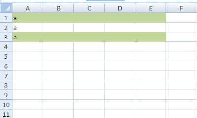
Occasionally there is a need when formatting a worksheet to use banded rows (i.e. cells in the odd rows color filled and the cells in the even rows not filled).  If the worksheet has only a few rows you can simply select the cells in the appropriate rows and format them with the desired color.  However, that's not practical when the sheet contains dozens or hundreds of rows.  When you have too many rows to do manually you can use conditional formatting.


Select the range of cells to which the formatting is to be applied.  For this example I've used the range A1:E10.

For Excel 2007 from the Home tab select Conditional Formatting > New Rule > "Use a formula to determine which cells to format".  Type the following formula in the "Format values where this formula is true" box:


=MOD(row(),2)


Click the Format button and select the Fill tab and then select the fill color.

Click OK

Click OK and your worksheet range now has banded rows.

In the future we'll look at how to make the rows dynamic so when you add data to rows after row 10 the conditional formatting will expand to the newly populated rows.


As always if you have any comments or questions, please comment here or email me at the office.

Prevent Selection Based on Value in Another Cell (cont.)

In the previous post we looked at using conditional formatting to "hide" selections in a cell based on selections made in another cell and in this post we'll use conditional formatting to provide the user with cells for data entry based on the selections in those same cells.


In the image below the selection for "MyHD Software" has been changed to "Y". When "Y" is selected the user is required to provide additional information for "Num Users" and "# Locations".  Since the user has not entered "Y" for "RF Warehouse Manager (w/HD)" the cells for "Num Users" and "# Locations" are filled Black.  If "MyHD Software" is "Y" then "RF Warehouse Manager (w/o HD)" is not available and is filled Black.

If the user has selected "Y" for "RF Warehouse Manager (w/o HD)" the "Num Users" and "# Locations" are still required and entries for "MyHD Software" and "RF Warehouse Manager (w/HD)" are invalid.

"Num Users" is in cell D7 and contains the formula =IF(OR(C8="Y",C10="Y"),"Num Users","") which displays the heading when either "MyHD Software" or "RF Warehouse Manager (w/o HD)" has been selected with a "Y".  Cell E7 uses the same formula with "# Locations" substituted for the text =IF(OR(C8="Y",C10="Y"),"# Locations","").


The range $D$8:$E$9 have two conditional formats applied (below).  The first fills the cells Black when "RF Warehouse Manager (w/o HD)" is selected ($C$10 = "Y").  The second places a single line border around the cells in the row where a "Y" is entered in column "C" (i.e. when "Y" is entered in cell C10 as above then cells D10 and E10 have single line borders.  The range of cells D8:E9 do not have single borders but this is not seen because they are filled Black).

The end result is that the user is presented with cells for data based on the selections made in column C.


Unfortunately, filling a cell Black does not prevent a user from entering a value.  Below is how our example displays if the user selects "Y" from the drop down in C9 when "N" is selected in C8.  Normally a user will not do that simply because it "appears" that a selection cannot be made in this cell but there is actually nothing preventing it being done.

To prevent this we can change the values available in cell C9.  In the example above the Data Validation below is used and provides a list of Y and N for the drop down.

We can use a dynamic list of values in order to limit the available selection.
In cell M1 the heading "List" is entered.  The formula =IF(C8="N","N","Y") is entered in cell M2 and =IF(C8="N","","N") is entered in M3.  When the value in C8 = "N" cell M2 will = "N" and M3 will be blank.  When the value in C8 = "Y" then cell M2 will = "Y" and M3  will = "N".


Next we want to adjust the length of our "list" to match the entries.  In cell L1 the heading "List Len" was entered.  Cell L2 contains the formula =IF(C8="N",1,2) which results in a value of 1 when C8 = "N" and a value of 2 when C8 = "Y".


Now we create a dynamic named range.  For Excel 2007 select the Formulas tab and then Define Name.  For Excel 2003 and earlier select Insert > Name> Define to display the New Name box.  Enter the desired name (I used validList) and then enter the formula =OFFSET($M$2,0,0,$L$2,1) and click OK.

The Data Validation for cell C9 was opened and changed from Y, N (above) to use the named range validList as below.

Now when the value in cell C8 = "N" the drop down in cell C9 only displays a  value of "N" but when C8 = "Y" the drop down in C9 displays "Y" and "N".

As always if you have and questions or comments regarding this post, please, comment here or email me at the office.

Prevent Selection Based on Value in Another Cell

I've been working on a workbook for our Sales Department that contains an element that might be of interest especially if your company uses Excel workbooks for inputting data rather than just using it to extract data from your ERP database.

One of the purposes of this to allow the selection of options regarding the HD software and our Value Add Products.  The selection values for all the products is a simple Y/N but based on the selection of a particular product other selection options may change (i.e. If MyHD Software is selected the user cannot select "RF Warehouse Manager w/o HD").  Additionally some selections require additional fields for input of data to be displayed.

The image below has all options set to "N".  Since the user should not be able to select "RF Warehouse Manager (w/HD)" if the "MyHD Software" had not been selected conditional formatting has been used to prevent the user from "seeing" the cell.  

If you're using Excel 2007, on the Home tab click Conditional Formatting > New Rule > Use a formula to determine which cells to format.  In this case the we want to condition the Y/N cell related to RF Warehouse Manager (w/HD) to be dependent on the Y/N entry for MyHD Software so we enter the formula =C8="N".  Now click the "Format..." button and from the Fill tab select Black and click OK.

If you're using Excel 2003 click Format > Conditional Formatting

Click the drop down and select "Formula Is".  Enter the formula =C8="N".  Click the "Format..." button and from the Patterns tab select Black.  Click OK and then click OK again.

Now whenever the condition C8="N" evaluates to True the cell will be Black.

I've used this method of prevention many times and it works okay but does not actually prevent the user from entering or selecting a value in the target cell.  If you want to prevent the user from entering an invalid entry in Cell C9 you can use a Dependent Drop Down List.  This presents the user with a drop down list in cell C9 that is dependent on the value in cell C8.  

We'll look at how to do that in the next post.

As always, if you have any comments or questions (no one ever does) you can  comment here or email me.

Formula used to Calculate Date Range

Wow...I can't believe it's been almost a month since the last posting.  Even those there's been a lot going on at work (i.e. new projects, a new customer, existing projects) there's just no excuse to not keep up with these postings since there are so many people reading the blog.  I know this only because of the stats tracked by the site not because of any feedback or comments because there are none of those.  


So to pick back up where we left off we'll take a look at the formula used to allow a user to select a fiscal year and the workbook will display data based on the selection.  The user wanted to be able to select a year from a drop down and have data display for that period for both the current and previous fiscal year.  Since that posting I've had a similar request but this user wants to be able to select a year and if it's a previous year display data for the entire year but it the current year is selected display data through the last full month.  The formula used for the beginning of each of these is the same.


We'll begin with a look at the layout of the dates for a five year period (below).  First we need a formula for the "Begin Date" of the current fiscal year in cell R6.  The formula used in this example is:
=IF(MONTH(TODAY())<3,DATE(YEAR(TODAY())-1,2,1),DATE(YEAR(TODAY()),2,1))
Since this customers fiscal year runs February through January then we have no current fiscal year data until we are in the month of March so the formula if the current date is less than month 3 (i.e. March).  After March it will display the current year.

 The "End Date" for the current year is created with this formula:
=DATE(YEAR(TODAY()),MONTH(TODAY())-1,1).  This formula displays the first day of last month.


Next we want to display the Begin and End dates for the previous four fiscal years.  For the "Begin Date" in cell R5 we use this formula =EOMONTH(R6,-12) and then copy and paste the formula in range R2:R4.  If you're not familiar with this formula the arguments for it are =EOMONTH(base, offset) where the base value is a date from which the function should do its calculations, and the offset is a number that indicates how many months from the base date should be used.  The offset can be either positive or negative. 


For the "End Date" in cell S5 the same formula is used except our offset is a negative one (i.e. =EOMONTH(R6,-1)).  This formula is then copied and pasted to Range S2:S4.


Now that we have our table of dates we need to convert the dates into formats that can be used for the date selection as well as formats that can be passed to MS Query to return the correct data.


For the current fiscal year in cell T6 we use =YEAR(R6).  This formula is copied and pasted into range T2:T5.  The formula used for the Begin date in cell U6 is =YEAR(R6)*100+MONTH(R6).  This formula is also copied and pasted into range R2:R5.  For the End dates the formula is =YEAR(S6)*100+MONTH(S6).  As previously this formula is copied and pasted in range S2:S5.

The range T2:T6 is Named and used with either Data Validation or as in this case with a List Box from the Forms Control selection.  The Begin and End dates are used as the criteria for the MS Query.


In the case above where the customer wanted the MS Query to return data of any fiscal year selected only through the previous month related to the run date of the report we change the formula in cell S5 to =EOMONTH(S6,-12) and then copy and past to range S2:S5. This results in the table below:

As always, if you have any questions or comments you can leave them here as a comment or email me at randomexcel@att.net.

Calculate Date Range for Workbook Fiscal Year

I recently created a workbook for a customer that uses Year To Date data.  The report was made simpler because the customer did not want to use the current month so there was no need to calculate the percentage of the current months work days and then apply that percentage to the current month last year.  As with most workbooks the desire here was to automate as much of the data retrieval as possible and this included passing the MS Query the date range for which the query is to be run when the workbook is opened.  

The Fiscal Year runs from February through January.  From March through December the calculation is easily calculated using the DATE and TODAY functions like this for the beginning date =DATE(YEAR(TODAY()),2,1).  This returns February 1st for the current year.  The calculation for the ending date would be =DATE(YEAR(TODAY()), MONTH(TODAY())-1,1).  This formula returns the first day of last month which is what we want since for our purposes the Year To Date excludes the current month.

These simple formulas work great until the beginning of the new year.  In January 2012 the above formulas would produce the following date range February 1, 2012 to December 1, 2011 which is obviously not a valid date range.  February also produces an the invalid date range of February 1, 2012 to January 1, 2012.

Looking at these date ranges also brings up the question of what date range should be used when the workbook is run in February of any given year?  In February the customer wants to see February of the previous year through January of the current year.  In March the date range would be use February only (i.e. February through February).

Additionally the workbook compares data for Year To Date vs. Year To Date Last Year so its necessary to come up with formulas to calculate the beginning and ending date for the previous year.

So, now all you have to do is come up with formulas for the date ranges for the Current Year and the Previous Year.

In the next post I'll show you the formulas that I used in the workbook.

As always, if you have any questions or comments you can leave them here as a comment or email me at randomexcel@att.net.

Cost Overrides on Purchase Orders (cont)

In the workbook for the Cost Overrides the customer needs an easy way to compare the cost of an Item that has had the cost overridden with the Replacement Cost from the current price sheet.  To accomplish this add a new MS Query over the Price Sheet Detail file (PRPMPSD).  Additionally we want to provide the Vendor Name from the Vendor Master file (APPMVEN) and fields from the Vendor Price Sheet Master file (PRPMPSM).

  

We'll return the following fields to our worksheet: Vendor Number, Price Sheet Number, Manufacturer Number, Replacement Cost, Price Sheet Master Type and the Price Sheet Control Number.

The criteria for the query will be PRCD21 = 'C' (we only want to return Price Sheets that are Current) and IVNO07 = [itemnum] (using the brackets allows a value to be passed from the workbook back to MS Query).

The P/S data returned by the query looks this on my worksheet after formatting.

Passing the item number to the query is done from the Main worksheet by selecting a cell in the Item Number column and clicking the "Display Selected Item" button. 

Clicking the button runs code that copies the active cell, selects the Price Sheet Detail worksheet and pastes the Item Number into Cell R5 (row 5 is hidden in the previous screen print).

Now in the Parameters dialog box select the "Get the value from the following cell:" radio button.  Enter the cell reference in the box (the best way to do this is click in the box and then click cell C5).  Click the "Refresh automatically when cell value changes" check box.  Click OK.

Now whenever a new item is selected from the main worksheet and the button is clicked  the query will run and display data for the selected Item Number.

Here's the code used by the "Display Selected Item" button.

This code is used by the "Exit" button to return the user to the Main worksheet.

 

In the next post we'll cover additional enhancements that were requested for this workbook

As always, if you have any questions and/or comments either leave it here as a comment or email me at randomexcel@att.net.

New Email Address

If you would like to email me you can use the following email address:

randomexcel@att.net

Cost Overrides on Purchase Orders

This week I had a request from a customer for a workbook to display all Purchase Order line items that have had the cost overridden.  This post will detail the construction of that workbook.

When beginning a project you need to determine as closely as you can exactly what the person requesting the workbook want but frequently you'll find that even though they "think" they know what they want you will end up making additions or changes to the workbook before you complete the project.  Just be aware that the better your understanding of what the end user wants/needs the easier the project will be.

When starting on a new workbook I usually begin by entering the headings based on what the user has requested.  You need to consider the fields that will be used to populate the data for each heading and make additional fields that will be used but not displayed in your workbook (i.e. dates will display in one cell in Excel but require three or four fields from the HD database).  This workbook has no such requirements but it should be kept in mind.  The image below shows the worksheet with the headings entered.

Now we select cell B6 and create the MS query to return the data to the worksheet.  Based on the headings we will be extracting data from the Purchase Order Line Item File (POPTRL) and the Item Master File (IVPMSTR).  These two files are joined on the Item Number field (IVNO07).  The worksheet does not display a date but a date is used as part of the record selection process.  The date that will be used is the Last Update date.  For the date selection criteria the HD fields are joined to create a single field that can be passed as a parameter to the query.  Since date fields in HD are numeric this is accomplished by summing the fields like this: POCC01*1000000+POYR01*10000+POMO01*100+PODY01.  This result of this formula for July 1, 2011 is 20110701 which can be passed to the query to return records for the requested date.  The value for the date is set in brackets so it can be changed from the worksheet (i.e. [chgdate]).  Since the user is only interested in records where the cost has been overridden then the criteria also includes the Line Item Cost Override Code (POCD17).  After including the criteria and selecting the fields to be returned to the worksheet the query will look like this:

When the query is run to return the data to the workbook a dialog box will display requesting the parameter (date) to be passed to the query.  Enter the desired date and click OK.

The data is now returned to the worksheet as below:

NOTE: Since this is data from a Customers Production the Product Numbers have been blanked out.

Now add a heading for the date select in cell D4 (i.e. Enter Date >>) and enter a date in E4.  In cell M6 enter this formula - =SUM(YEAR(E4)*10000+MONTH(E4)*100+DAY(E4)).  This formula provides a field that will be used as the parameter for the query.  Now open the Parameter dialog box.  To open the dialog box in Excel 2007 click Data Tab > Connections  and select the query and click Properties > Definition Tab > Parameters button; for 2003 select a cell in the data returned by the query and right click and click Parameters.  In the Parameters dialog box

click the radio button "Get the value from the following cell:" and the check box "Refresh automatically when cell value changes".  Click in the field below "Get the value..." and then click in cell M6.  Click OK.  Now when the user changes the date in cell E4 the query will run and return data for the entered date.  Test the workbook to verify that it functions correctly and returns the correct data.

Lastly format the workbook as desired and test once more and it should be ready for your user.

Here's my formatted worksheet.

As always if you have any comments and/or questions leave a comment here or email me at the office.