More On Using Radio Buttons

In the last post I failed to include how to add Radio Buttons in Excel 2003.  Select the worksheet where the buttons will be used and click View > Toolbars > Forms.  The toolbox below appears as a floating toolbar.

Then proceed as with Excel 2007.


Another thing that will come up when you begin using control buttons will be the need to use more than one set of buttons.  As we've seen multiple buttons use the same Cell Link and the number in the cell corresponds to the button that is active.  So whether you have two or twenty buttons they will all use the same cell and will increment based on the total number of buttons.


In order to have multiple sets of buttons it's necessary to use the Group Box from the Forms toolbar (below).

Click on the Group Box and then click on the worksheet and adjust the size of the box to include the buttons that are to be grouped together as below where buttons 1 & 2 are inside Group Box 6.

Buttons 1 and 2 can now be assigned to a different Cell Link.  Any buttons outside the Group Box can now be assigned to a different cell and will work independently of the buttons inside the box.

As always if you have any comments or question you can leave them here or email me at the office.

Using Radio Buttons to Change Displayed Data

The vast majority of the workbooks that I do for customers are not printed but are used to interactively display data.  A good example of this would be a workbook that displays Sales data by Branch.  Select a Branch and Period and the workbook displays the data change the Branch and data for the new Branch is displayed.  There are occasions where the user wants to be able to easily change the data that's being displayed from one type to another.  An example would be providing the ability to switch between Gross Margin based on Replacement Cost and Gross Margin based on Weighted Average Cost.  One way to accomplish this is by using Radio Buttons.  Excel has two different types of Radio Buttons, Active-X and Forms; we'll be looking at the Forms type in this post.


We'll use the table below as the data source for our workbook

Select another worksheet and for Excel 2007 click the Developer tab and then from the Controls section click Insert and then click the Radio Button (Option Button) under Forms Control.

Click on the active worksheet in the general area where you want the Radio Button and Excel will create the Button as below.  For our purposes we'll not use the Caption so right click on the Button and select Edit Text and delete the text.

Right click and Copy the Button then right click and Past to create a second Button.

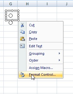
Right click on one of the Buttons and click Format Control.

Click in the Cell link box and then click in cell L2 and then click OK.  This links the buttons to cell L2.

Now, click one of the buttons and a number will appear in cell L2.  Click the other button and the number will change.  Since we have two buttons the numbers will be 1 and 2 and will change depending on the button that is active.  We can now reference cell L2 in a formula in order to display different results for our worksheet.


In cell B2 enter "Sales".  In cell B3 enter =Sheet1!A2 and then copy to cells B4 and B5.  In cell C3 enter =IF($L$2=1,Sheet1!D2,Sheet1!E2) and then copy to cells C4 and C5.  In cell D3 enter =IF($L$2=1,Sheet1!F2,Sheet1!G2) and copy to cells D4 and D5.  Format the data as desired and you should have something like this:

Since the data can change then we need to change the headings to match.  In cell C2 enter ="GM$ at "&IF($L$2=1,"RC","WAC") and in cell D2 enter 
="GM% at "&IF($L$2=1,"RC","WAC").  In cells H2 enter "Replacement Cost" and in cell H3 enter "W.A.C."


Format the headers as desired and you should have something similar to this:

As always, if you have any questions or comments leave them here or email me at the office.

Import JE Data into MyHD

One of the great new features in MyHD is the ability to easily import Journal Entry Data.  The user enters the G/L Account Number, Amount and Description in Excel and then saves as a .CSV file.  


The user simply navigates to the Journal Entry screen and enters the Journal Reference code and Reference Number then clicks OK.

The user now clicks the Import button

Selects the file to be imported

Click Open and the data is loaded to the JE

To make this process even simpler we've created an Excel workbook specifically for the data entry

This workbook has MS query that runs against the customers database and validates the G/L Accounts plus a formula to indicate that the data is in balance.  When the data entry is completed the user clicks the "Crt CSV" button and the data is copied to a new workbook which is then saved on the users C drive.

We also have a workbook for loading JE Data to the database for customers that are still using HD.  Since there is no Import feature in HD the data from the workbook is loaded to the database via Client Access.

If you would like a copy of either of these workbook send me an email and I'll forward it to you.

As always if you have any questions or comments you may post them here or email me directly.

Date Selections for HD Parameter Queries

I receive frequent requests for reports that require the user to provide a from and to date to the MS Query.  Ideally you would like to prevent the user from receiving an error message because a to date that is less than the from date is entered.  There are several way of accomplishing this and here is the one that I prefer.


Here's the layout of our sample workbook.

The todate list (column B) is built by entering =TODAY() in cell B13 and then entering =EOMONTH(B13,-1) in cell B12.  The formula in B12 is then copied and pasted in range B2:B11.  This populates the range B2:B12 with the last day of each month for the  previous 11 months.

The fromdate list (column A) is built by entering =DATE(YEAR(B2),MONTH(B2),1) in cell A2.  The formula is then copied  and pasted in the range B3:B13.  This populates the range A2:A13 with the first day of each month corresponding to the date in column B.

The Named Range "fromdate" is created by selecting the range A1:A13 and selecting  Formulas >  Create from Selection and clicking OK.

Select cell I2 and then Data > Data Validation and from the dropdown select List.  In the Source box enter =fromdate and click OK.  Cell I2 now has a drop down from which the user can select a date.  Format the cell with a date format.

Since the user should not be able to select a todate that is less than the fromdate it's necessary to determine where the todate list should begin based on the users selction for fromdate.  Enter =MATCH($I$2,$A$2:$A$13,0)-1 in cell E2.  The arguments for the MATCH formula are lookup_value, lookup_array, match_type.  The formula looks for the selected From Date (I2) in the list of From Dates (A2:A13) for an exact match (0) and returns the relative position of the cell where the match is found.  The -1 is used because the offset formual that will be used for the name range begins in row 2 instead of row 1. 

In cell E3 enter the formula =12-E2.  This will be used in the offset formula to determine how many cells to display. 

Select cell B2 then Formulas > Define Name and in the Name box enter todate.  In the Refers to: box enter =OFFSET(Sheet1!$B$2,Sheet1!$E$2,0,Sheet1!$E$3,1) then click OK.  The arguments for OFFSET formula are reference, rows, cols, height, width.  The reference is the cell address from which the offset will occur (B2).  Rows is the number of rows to offset from the reference cell, in this case it's the value in cell E2.  Columns is the number of columns to offset from the reference cell, in this case the value is 0 since we do not want a column offset.  Heighth  is the number of rows to be returned, in this caase we use the value in cell E3.  Width is the number of columns to be returned, in this case we only have the single column of data so we use 1.

Select cell I3 and then Data > Data Validation and from the dropdown select List.  In the Source box enter =todate and click OK.  Cell I3 now has a drop down from which the user can select a date that is always greater than or equal to the From Date.  Format the cell with a date format.

Cells K2 and K3 contain formulas to convert the dates to a format that can be used as parms for the MS Query .

  =SUM(YEAR(I2)*10000+MONTH(I2)*100+DAY(I2))

As always if you have any comments or questions you can enter them here or email me at the office.  Also, if you would like to have the sample workbook send me an email and I'll send it to you.